Run Amplitude Change Detection (ACD)
Lesson 1 of 1
Run Amplitude Change Detection (ACD)
In this quick guide, you will:
- •
Learn how ACD is used to monitor large-scale changes that occur across broad geographic regions. * •
Open and display two overlapping Single Look Complex (SLC) images of a port in the Bay of Gibraltar from different dates. * •
Create an ACD classification image that reveals changes in vessel positions during an eight-day period.
Sample Data
The exercises in this quick guide use two Capella SLC images for demonstration. Download the ZIP file below and extract its contents to a directory on your computer.
[SAREssentials_ACD.zip
1.1 GB
DownloadArrow down with horizontal line beneath it](assets/SAREssentials_ACD.zip)
- •
File names: Capella_Gibraltar_2021-07-30_slc and Capella_Gibraltar_2021-08-07_slc. ENVI header files (.hdr) and ENVI SARScape files (.sml) are also included. * •
Acquisition dates: 30 July and 7 August, 2021 * •
Processing notes: The source datasets were Sensor Independent Complex Data (SICD) files in National Transmission Imagery Format (NITF), which require the ENVI NITF/NSIF Module to read. Since not all users have the ENVI NITF/NSIF Module, we used the "Imported data" option in the SAR Basic Data Processing tool to create SLC images that are in SARscape format instead of SICD. * •
Source: Capella Space Open Data(opens in a new tab), Attribution 4.0 International (CC BY 4.0)(opens in a new tab) license. The source IDs are CAPELLA_C03_SP_SLC_HH_20210730095929_20210730095932 and CAPELLA_C03_SP_SLC_HH_20210807095836_20210807095839.
Background
Amplitude Change Detection (ACD) examines the backscatter ratio between two amplitude images from different dates. In an ACD image, blue pixels indicate new features, while red pixels indicate features that are no longer present. ACD is best used for large-scale changes that occur across broad geographic regions.
Data Requirements
SLC images used for ACD must have the same:
- •
Frequency * •
Polarization: VV, HH, VH, or HV * •
Orbital direction: ascending (North-South flight) or descending (South-North flight) * •
Acquisition mode: i.e., spotlight (preferred), stripmap, sliding stripmap, dwell, etc. * •
Incidence and azimuth angles: No more than 3 degrees difference
ACD works with magnitude or power data, which can be derived from ingested SLC data or power images in slant- or ground-range geometry. The other two workflows (CCD and ACD+CCD), which are based on coherence products for classification, only accept SLC input data since they rely on both magnitude and phase.
Tip: To check if your images are suitable for ACD, run the SAR Compatibility Check tool in the SAR Essentials folder of the Toolbox. See the SAR Essentials: Check Data Compatibility quick guide for more information.
Open and Display Capella SLC Images
- 1
Start ENVI. - 2
Select File > Open from the Menu bar. An Open dialog appears. - 3
Use the Ctrl key to multi-select the following files, then click Open:
Capella_Gibraltar_2021-07-30_slc
Capella_Gibraltar_2021-08-07_slc
- 4
Wait for the raster pyramids to build in the Status bar, then click the Zoom to Full Extent button in the Toolbar. Both images are displayed at their full extent. In the following screenshot, the July 30 image is displayed first:

Both images cover part of the Bay of Gibraltar east of Algeciras, Spain. The images are flipped along the North-to-South direction because they were acquired from descending (South-to-North) orbital passes.

Google Earth imagery shows that this is a commercial port with cargo ships and shipping containers.

Like other SLC images, the Capella images represent slant-range geometry and have not been georeferenced or corrected for terrain effects. They are suitable for ACD since their incidence angles vary by only 1.3 degrees and their azimuth angles vary by 1.2 degrees.
Run the SAR Amplitude Change Detection Tool
- 1
Go to the Toolbox and expand the SAR Essentials > Change Detection folder. - 2
Double-click SAR Amplitude Change Detection. The SAR Amplitude Change Detection tool appears. The Input tab is active.
Select Input Files
- 1
Click the Browse button next to Before Image. A file selection dialog appears. - 2
Select the file Capella_Gibraltar_2021-07-30_slc.sml and click Open. - 3
Click the Browse button next to After Image. - 4
Select the file Capella_Gibraltar_2021-08-07_slc.sml and click Open. - 5
Leave the Spatial Subset field blank. This is for selecting a pre-defined shapefile of the area of interest. You will process the entire images instead.

- 6
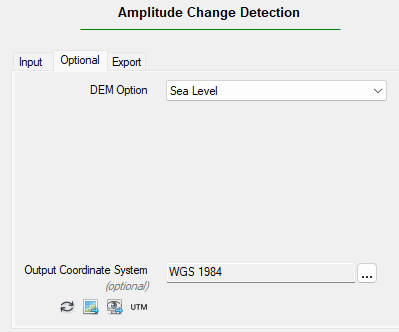
Click the Optional tab. - 7
Click the DEM Option drop-down list and select Sea Level. - 8
For the Output Coordinate System, leave the default value of WGS 1984.
Set Export Options
- 1
In the Grid Size field, enter a value of 3 meters. Although the Capella image resolution is about 0.5 meters, increasing the Grid Size to 3 meters will speed up processing and reduce noise in the final result. - 2
In the Generate Products list, select Filtered Classification. - 3
The filtered classification image will be written to the directory specified in the ENVI Output Directory preference. To specify a different output folder, click the Browse button next to Output Folder and choose a different folder.

- 4
Click the Next button. Processing takes several seconds to complete. When it is finished, a temporary change detection image is added to the Layer Manager and displayed in the Image window. The ACD tool advances to the Change Detection Threshold step. The ACD process is not yet complete; you will need to review the change detection image and determine suitable threshold settings next. - 5
In the Layer Manager, uncheck both Capella images to hide them. Only the change detection image is displayed.

Review the Change Detection Image and Threshold Setting
Red pixels indicate features that are no longer present on August 7, while blue features indicate new features on August 7.
The Amplitude Ratio Threshold value determines how much change the classification image should show. Increasing the threshold value will show the highest amounts of change in the intervening time period, while suppressing background noise.
- 1
Set the Amplitude Ratio Threshold value to 9, then click Next. The Classification Smoothing panel appears, and a classification image is displayed. - 2
Look at the Layer Manager and notice that the classification image has four classes: “Unclassified” (black), “No Change” (gray), “Increment” (blue), and "Decrement" (red).
The "Increment" class represents new features on August 7, while the "Decrement" class represents features that were present on July 30 but not August 7.

Smooth the Classification Image
This step is optional; You can clean up the classification image by filtering out small groups of pixels and aggregating the remaining pixels into clusters. This step removes most of the speckled noise that you see in the initial classification image.
- 1
The defaultKernel Size value is 3. Enable the Preview option to see what the final classification will look like with this value. The edges of features are sharp and noisy. Small groups of isolated pixels appear in the image. - 2
Set the Kernel Size value to 7with the Preview option still enabled. The objects are much smoother; however, they lose their original shape and detail.

- 3
Disable the Preview option. - 4
Set the Kernel Size value to5, then click Next. The Report panel is displayed. - 5
Click Finish. Two new layers are added to the Layer Manager and displayed in the Image window:
- •
acd_ann_info.anz: Annotation layer showing the line-of-sight (range) and heading (azimuth) directions, along with basic metadata. You must zoom out of the view to see the annotation layer, which is displayed to the upper-right of the classification image. * •
change_detection_map_fil.dat: Smoothed/filtered classification image

This concludes the quick guide.
To summarize, an Amplitude Change Detection (ACD) image can provide insights into patterns of life and the movement of goods through an area. This exercise demonstrated how to create a change detection image that revealed vessel movement over an eight-day period. However, the image cannot definitively identify vessels or track their exact positions. Coordination with the Automatic Identification System (AIS) is needed for that. The AIS is a broadcast system that acts like a transponder on vessels. Monitoring and tracking vessels that broadcast AIS signals can verify which ones are operating legally.
Your input is important to us, please take a few moments to fill out ourQuick Guide Feedback(opens in a new tab)form.
© 2025 NV5 Geospatial Solutions, Inc. This information is not subject to the controls of the International Traffic in Arms Regulations (ITAR) or the Export Administration Regulations (EAR).