Create Digital Surface Models (DSMs) from Interferometry
Lesson 1 of 1
Create Digital Surface Models (DSMs) from Interferometry
In this quick guide, you will:
- •
Learn what factors contribute to the reliability of topographic height estimates. * •
Learn the data requirements of images used for interferometric DSM generation. * •
Use the SAR Interferometric DSM tool to create a DSM from two overlapping Single Look Complex (SLC) images acquired eight days apart. * •
Review other raster products created from the SAR Interferometric DSM tool.
Sample Data
The exercises in this quick guide use two Umbra SLC images for demonstration. Download the ZIP file below and extract its contents to a directory on your computer.
[SAREssentials_DSM_Interferometry.zip
884.9 MB
DownloadArrow down with horizontal line beneath it](assets/SAREssentials_DSM_Interferometry.zip)
- •
File names: Umbra_SaghandIran_2023-08-17_slc and Umbra_SaghandIran_2023-08-25_slc. ENVI header files (.hdr) and ENVI SARscape files (.sml) are also included. * •
Acquisition dates: 17 August and 25 August, 2023 * •
Processing notes: The source datasets were Sensor Independent Complex Data (SICD) files in National Transmission Imagery Format (NITF), which require the ENVI NITF/NSIF Module to read. Since not all users have the ENVI NITF/NSIF Module, we used the "Imported data" option in the SAR Basic Data Processing tool to create SLC images that are in SARscape format instead of SICD. * •
Source: Umbra Open Data Program(opens in a new tab), Attribution 4.0 International (CC BY 4.0)(opens in a new tab) license. The source IDs are 2023-08-17-05-53-58_UMBRA-05_SICD and 2023-08-25-18-47-23_UMBRA-06_SICD.
Background
Creating DSMs from interferometry involves determining the phase difference between two SAR images that mostly cover the same geographic area. This approach assumes that no terrain deformation has occurred between two satellite acquisitions.
The accuracy of the DSM depends on the spatial and temporal separation of the satellite positions at the moment of data acquisition, particularly the geometric configuration of the image pair in terms of normal baseline separation (which refers to the spatial separation between the two satellite tracks). A larger baseline separation improves the accuracy of the DSM estimation; however, it also increases the risk of processing errors.
A small temporal difference between acquisitions also results in better accuracy. By contrast, large temporal differences can introduce weather and seasonal surface changes--such as vegetation, snow, and ice--that reduce the accuracy of the generated DSM. This is especially true with high-frequency (X-band) sensors.
The reliability of DSM generation also depends on the interaction of the radar signal with the terrain, as well as the imaging geometry (baseline).
Radar Frequency and Terrain Implications
In SAR sensors with long wavelengths (for example, L-band and P-band), the radar signal penetrates through foliage and interacts with trunks and branches. In these areas, topographic estimation is slightly below the vegetation canopies. Thus, the output is not strictly a DSM as it would be with smaller wavelength sensors that operate in the X- or C-band.
One drawback with X-band data (such as Umbra or Capella) is with repeat-pass mode. Canopy cover often causes decorrelation, making the final measurement inaccurate or unreliable. In contrast, longer wavelengths provide a more coherent measurement but do not actually produce a surface model.

SAR penetration capabilities by wavelenth. Image credit: NASA Earthdata (2020).
Stereo radargrammetry DSM processing cannot be applied to interferometric acquisitions, regardless of the sensor used.
Data requirements
Both images used for interferometric DSM generation must meet the following requirements:
- •
They must be from the same sensor. * •
They must have the same geometry (ascending or descending). * •
They must be co-polarized (VV or HH). Co-polarized data have a higher phase signal-to-noise ratio and therefore provide more precise topography estimates. * •
They must be SLC datasets in slant-range geometry. Geocoded images are not allowed. * •
The ground footprint overlap area must be 80% or more. This overlap constraint also applies to any reference DEMs or shapefiles used to define spatial subsets. * •
The incidence and heading angles must be less than 1 degree. * •
They must respect the constraints of the maximum normal baseline (less than 60% of the critical baseline). * •
They must respect the contraints of the Doppler difference (less than 60% of the Pulse Repetition Frequency, or PRF).
Before creating an interferometric DSM, use the SAR Check Data Compatibility tool to check if your images meet these requirements. See the SAR Essentials: Check Data Compatibility quick guide for more information.
Next, you will generate a DSM from the same pair of Umbra images that were used in the SAR Essentials: Run Coherent Change Detection quick guide. The images are centered over the village of Saghand, Iran.
Run the SAR Interferometric DSM Tool
- 1
Start ENVI. - 2
Go to the Toolbox and expand the SAR Essentials > DSM folder. - 3
Double-click the SAR Interferometric DSM tool. The SAR Interferometric DSM dialog appears.
Set Input Options
- 1
Click the Browse button next to Reference Image. A file selection dialog appears. - 2
Go to the location where you saved the sample data for this quick guide. - 3
Select the file Umbra_SaghandIran_2023-08-17_slc.sml and click Open. - 4
For the Secondary Image, select the file Umbra_SaghandIran_2023-08-25_slc.sml. - 5
Leave the Spatial Subset field blank. This is for selecting a pre-defined shapefile or Google Earth KML/KMZ file delineating the area of interest. The Umbra images have already been spatially subsetted. - 6
In the Coherence Threshold field, enter a value of 0.5. This value specifies the level of quality and precision in the output DSM. Values can range from 0 (lowest quality) to 1 (highest quality). Pixel values lower than the specified coherence will not be considered for DSM generation.

Select a DEM
The use of a reference DEM is highly recommended, as it streamlines internal processing and helps avoid phase aliasing in areas with strong topographic variability. The higher the resolution and accuracy of the reference DEM, the better the quality of the output DSM.
For this exercise, you will use a 30-meter Shuttle Radar Topography Mission (SRTM) DEM that was converted to ENVI SARscape format. High-resolution reference DEMs are not available for this region.
- 1
Click the Optional tab. - 2
Click the DEM Option drop-down list and select Use Input DEM. - 3
Click the Browse button next to Input DEM and select the file SRTM DEM Iran.dat. - 4
Click Open. - 5
Select the Yes option for Subtract Geoid. - 6
Remove the default value of -32768 from the Data Ignore Vaue for DEM field. - 7
For the Output Coordinate System, keep the default value of WGS 1984.

Set Export Options
- 1
Click the Export tab. - 2
Leave the Grid Size field empty. ENVI will automatically determine a suitable output grid resolution based on the nominal resolution of the SAR imagery and an internally applied multilooking factor. - 3
Click the Select All button to the right of the Generate Products list. This selects all options.

- 4
The output rasters will be written to the directory specified in the ENVI Output Directory preference. To specify a different output folder, click the Browse button next to Output Folder and choose a different folder.

- 5
Click the Next button. Processing takes several minutes to complete. When it is finished, the Report panel appears and the output products are added to the Layer Manager and displayed in the Image window. - 6
Click the Finish button to close the tool.
Evaluate Output Products
The Layer Manager lists several new layers:
- •
dsm.anz: Annotation layer showing the line-of-sight (range) and heading (azimuth) directions, along with basic metadata. You must zoom out of the view to see the annotation layer, which is displayed to the upper-right of the DSM image in the Image window. * •
dsm.dat: DSM image * •
coherence_geo.dat: Geocoded coherence image * •
resolution.dat: Resolution image where pixel values represent spatial resolution, in meters * •
precision.dat: Precision image where pixel values represent the precision of height estimates, in meters

Let's look at each output product in more detail.
DSM
The DSM is the first layer displayed in the Image window. A DSM is different than a DEM or Digital Terrain Model (DTM) because elevation values include features that protrude from the surface. A DEM or DTM characterizes the topography of a bare Earth surface. A high-resolution DSM such as this one can reveal large vegetation canopies and buildings. Darker pixels correspond to lower elevation, while brighter pixels correspond to higher elevations.

Not all white areas indicate higher elevation values, however. When you set a Coherence Threshold value earlier, pixels with coherence values less than 0.5 were masked out of the coherence image and set to "No Data." The masked pixels are the same in every output product, including the DSM.
Tip: Viewing the DSM as a grayscale raster is not always intuitive, nor does it reveal masked pixels well. Consider using ENVI's Topographic Shading Tool to create a color shaded-relief image from the DSM. This is a good way to visualize elevation data. For more information, see the Topographic Shading(opens in a new tab) topic in ENVI Help.

Example of using the Topographic Shading Tool to view a shaded-relief image from the Iran DSM.
Once you create a DSM, you can use it for the following analyses:
- •
Topographic analysis * •
Viewshed analysis using ENVI's Viewshed Tool (accessible from the Toolbar) * •
Mobility analysis tools, such as Helicopter Landing Zones or Topographic Breaklines, which are both under the Mobility folder in the Toolbox.
- 1
In the Layer Manager, uncheck the dsm.dat layer to hide it. The coherence image is displayed.
Coherence Image
Coherence values range from 0 (low coherence, or unstable or non-reflecting areas) to 1 (high coherence, or stable areas). Thus, brighter pixels in the coherence image indicate stable areas, or those that did not change over time. Darker pixels indicate changes to the landscape that occurred during that time. Since you set a threshold of 0.5 earlier, pixel values below 0.5 are masked out and set to "No Data." These areas of extremely low coherence may be caused by excavation, soil disturbance, vehicle movement, and/or foliage impacted by wind and short-term growth.

The coherence estimates in this image are not highly precise. This approach only considers a limited number of pixels in order to preserve resolution, but as a statistical estimate, it is not reliable over small regions. Other techniques such as Coherent Change Detection provide a more accurate coherence estimation, although they are more time-consuming.
- 2
In the Layer Manager, uncheck the coherence_geo.dat layer to hide it.
Resolution Image
Pixel values in this image represent spatial resolution based on the local incidence angle. Darker values indicate finer spatial resolution, while brighter values indicate coarser resolution. As with the other output products, white areas indicate masked pixels.

- 3
Optional: In the Layer Manager, right-click on resolution.dat and select Quick Stats. The Statistics View dialog reports the minimum and maximum resolution values. - 4
Optional: Enable the Histograms option in the Statistics View dialog to better understand the distribution of pixel values, which are reported in the "DN" column. Most of the values range from 0.44 to 11.6 meters. Values higher than this (up to the maximum of 130.13 meters) are primarily outliers.

Refer to the Compute Image Statistics quick guide for more information.
- 5
Close the Statistics View dialog. - 6
In the Layer Manager, uncheck the resolution.dat layer to hide it.
Precision Image (precision.dat)
This image provides an estimate of the precision of height measurements, in meters. Lower pixel values represent higher precision, while higher pixel values represent lower precision. It is only an estimate derived from coherence and the acquisition geometry. It does not account for potential phase aliasing or phase bias that may occur during processing.

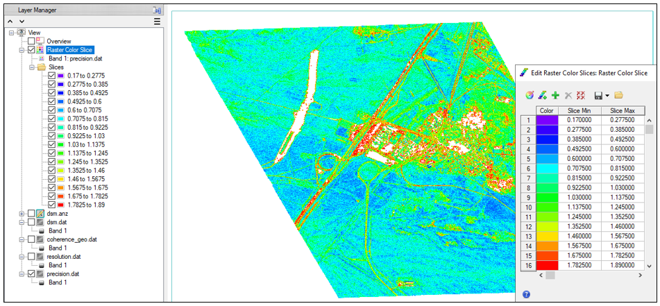
Viewing the image in color provides better insight to the overall precision. You can apply a raster color slice to do this.
- 7
In the Layer Manager, right-click on precision.dat and select New Raster Color Slice. The Data Selection dialog appears. - 8
Select Band 1 under precision.dat and click OK. The Edit Raster Color Slices dialog appears, and a raster color slice layer is added to the Layer Manager and displayed in the Image window.
Red and orange pixels indicate areas with lower precision. Blue pixels indicate those with the highest precision.
The precision layer closely mimics the coherence layer. Roads exhibit low coherence, which translates into poor precision and high uncertainty. They have low coherence and precision because they reflect poorly; their flat surfaces cause most of the signal to scatter away rather than return to the sensor.
Buildings show a different behavior, possibly influenced by nearby trees along the roads. Additionally, small changes in the incidence angle can cause directional reflections from objects, which can further reduce coherence.
The rest of the image mainly consists of dry, bare soil, which reflects the signal well, remains stable, and produces high coherence, resulting in good precision.
- 8
Click OK in the Edit Raster Color Slices dialog to dismiss it.
This concludes the quick guide.
Additional Resources
SAR Essentials: Create Digital Surface Models (DSMs) from Stereo Radargrammetry quick guide
Your input is important to us, please take a few moments to fill out ourQuick Guide Feedback(opens in a new tab)form.
© 2025 NV5 Geospatial Solutions, Inc. This information is not subject to the controls of the International Traffic in Arms Regulations (ITAR) or the Export Administration Regulations (EAR).