Perform a Supervised Classification

来源: https://vis-webcontent.s3.amazonaws.com/quickguides/Classification/Supervised+Classification/index.html#/

Lesson content

Lesson 1 of 1

Perform a Supervised Classification

In this quick guide, you will:

•

Open and display a Sentinel-2 layer-stacked image. * •

Restore a Region of Interest (ROI) file with training data for predefined classes. * •

Preview classification results from multiple supervised classifiers. * •

Run supervised classification and create an ENVI classification raster and shapefile. * •

Edit the shapefile properties so that each class has a unique line and fill color.

Sample Data

Download sample data below. Then extract the contents of the .zip file to a local directory.

[Sentinel2_LandCoverClassification.zip

1.7 GB

DownloadArrow down with horizontal line beneath it](assets/Sentinel2_LandCoverClassification.zip)

Background

When you are familiar with the area covered by a scene and you know what features it contains, you can perform a supervised classification.

A key component of supervised classification is the use of training data to provide examples of the features you are interested in. These examples have a known identity because they were selected from the image (or in the field) with a high degree of certainty that they correspond to specific features. Classification algorithms then use the spectral properties of the training data to classify pixels of unknown identity into one of the classes you defined. Training data can come directly from image pixels. In ENVI, you can collect training data from image pixels using ROIs.

Open and Display a Sentinel-2 Multispectral Image

1

Select File > Open from the Menu bar. An Open dialog appears. 2. 2

Go to the location where you saved the sample data, and select the file Sentinel2_LayerStack_Montana.dat. 3. 3

Click Open. The image is added to the Layer Manager and displayed in the Image window. 4. 4

Click the Zoom to Full Extent button in the Toolbar.

This is a layer-stacked image, which means that the 10-meter and 20-meter multispectral bands were combined in one image rather than in separate band groups. See the Build Band and Layer Stacks quick guide for more information.

Start the Classification Workflow

1

In the Toolbox, expand the Classification folder and double-click Classification Workflow. The workflow begins with the File Selection panel. The Raster File field is already populated with Sentinel2_LayerStack_Montana.dat 2. 2

Click the Next button to proceed to the Classification Type panel. 3. 3

Select the Use Training Data option, then click the Next button to proceed to the Supervised Classification panel.

Restore a Training Data ROI File

For this exercise, you will classify different land-cover types using the U.S. Geological Survey's LCMAP Level-1 scheme(opens in a new tab). The land-cover types include Developed, Cropland, Grass/Shrub, Tree Cover, Water, Wetland, Ice/Snow, and Barren.

Level 1 LCMAP land-cover classes. Source: U.S. Geological Survey, public domain.

You will restore an ROI file with training data for each feature class that has already been created for you. See the Collect Classification Training Data From Image Spectra quick guide for an example of how to create such a training data ROI file.

1

Click the Load Training Data Set button.

The Select Training Data File dialog appears.

2

Go to the location where you saved the sample data, and select the file TrainingDataROIs.xml. 2. 3

Click Open. The ROIs are listed in the Classification Workflow, added to the Layer Manager, and displayed over the Sentinel-2 image.

4

In the Layer Manager, uncheck the Regions of Interest folder to hide the ROIs.

Next, you will preview classification results from four different supervised classifiers.

5

Click the Algorithm tab. 2. 6

Click the drop-down list above Probability Threshold, and select Minimum Distance.

Minimum Distance Classification

A Minimum Distance classifier is the foundation for other supervised methods. It calculates the Euclidean distance between each pixel and the mean vectors of each class, then it assigns each pixel to the nearest class. It is reasonably fast. It classifies every pixel in the image up to a specified maximum distance or standard deviation threshold.

1

Enable the Preview option. A Preview portal appears in the Image window. It shows the results of Minimum Distance classification with no standard deviation or maximum distance set. 2. 2

Click the Select button (the arrow icon) in the ENVI Toolbar. 3. 3

Move the cursor to the top of the Preview Portal until a four-sided arrow icon appears. Then click and drag the Preview Portal to move it around around the Image window. 4. 4

To enlarge the Preview Portal, click and drag its lower-right corner to expand it.

5

Move the cursor to the top of the Preview Portal to display the toolbar, then select the green Play button. The Preview Portal flickers between the classification result and the Sentinel-2 image. This is a convenient way to compare the two images. 2. 6

To stop the flicker, click the Pause button in the Preview portal toolbar. 3. 7

Click the Single Valueradio button under Standard Deviations from Mean. The default value is 10,000,000. 4. 8

Change the Standard Deviations from Mean value to 3, and press the Enter key. The Preview portal updates accordingly. Pixels whose reflectance values exceed three standard deviations beyond the class means (for all classes) are unclassified. They are the black pixels you see in thePreview portal. The lower the value, the more pixels that are unclassified.

Instead of using standard deviation as a threshold, you can specify a maximum distance from class means.

9

Click the None radio button under Standard Deviations from Mean. 2. 10

Click the Single Value radio button under Maximum Distance Error. Again, the default value is 10,000,000. 3. 11

Change the Distance Error value to 2000, and press the Enter key. Pixels whose Euclidean distance is more than 2,000 pixels from the class means (for all classes) are unclassified.

12

Move the Classification Workflow out of the way, then move the Preview portal around the Image window to review the classification results in different areas.

Tip: To zoom out while the Preview portal is active, click once in the Image window and use the scroll wheel on your mouse to zoom. Click and hold the scroll wheel or middle mouse button to pan around. You may experience slight delays while the Preview portal is updated.

Notice the increased misclassification of pixels in the mountainous areas. Pixels under shadow are incorrectly classified as "Water." Bright pixels are incorrectly classified as "Developed."

Let's try a different supervised classifier.

Maximum Likelihood Classification

This classifier assumes that the statistics for each class in each band are normally distributed. It calculates the probability that a given pixel belongs to a specific class. Each pixel is assigned to the class that has the highest probability.

1

Click the drop-down list of classifiers and select Maximum Likelihood. The Preview portal updates accordingly.

2

Click the Single Value radio button under Probability Threshold. 2. 3

Experiment with different Probability Threshold values between 0 and 1. The threshold is a probability minimum for inclusion in a class. For example, a value of 0.9 will include fewer pixels in a class than a setting of 0.5, because a 90% probability requirement is more strict than allowing a pixel in a class based on a chance of 50%. 3. 4

Use the flicker operation in the Preview portal to compare the classification result with the Sentinel-2 image. Maximum Likelihood classifies many more pixels was "Water," compared to Minimum Distance. Also, the water pixels are small and scattered, which is not correct.

Mahalanobis Distance Classification

This classifier is similar to Maximum Likelihood, except that it assumes all class covariances are equal, and therefore is a faster method. Like Minimum Distance, it calculates the Euclidean distance from each unknown pixel to the mean ROI for each class.

1

Click the drop-down list of classifiers and select Mahalanobis Distance. The Preview portal updates accordingly. 2. 2

Click the Single Value radio button. 3. 3

Change the Distance Error value to 5, and press the Enter key.

The **Distance Error** parameter works a little differently, compared to the Minimum Distance classifier. Mahalanobis Distance accounts for possible non-spherical probability distributions. The **Distance Error** is the distance within which a class must fall from the center or mean of the distribution for a class. The smaller the distance threshold, the more pixels that are unclassified.

In the agricultural region, Mahalanobis Distance classifies more pixels as "Wetland," compared to Minimum Distance or Maximum Likelihood. Also, the agricultural region shows more variability between classes when compared to the other two methods.

Spectral Angle Mapper Classification

SAM uses an n-Dimensional angle to match pixels to training data, where n is the number of spectral bands. It compares the angle between the training mean ROI and each pixel ROI in n-D space. Smaller angles represent closer matches to the reference spectrum. The pixels are classified to the class with the smallest angle.

1

Click the drop-down list of classifiers, and select Spectral Angle Mapper. The Preview portal updates accordingly. Notice that fewer pixels are misclassified as "Water" in the mountains areas, compared to the other three classifiers.

2

Click the Single Value radio button. 2. 3

Experiment with different Spectral Angle values between 0 and 1.5708 (Pi/2) radians. This is the angle within which a pixel resides to be considered part of a class.The lower the value, the more pixels that are unclassified. The following screenshot shows an example of setting the Spectral Angle to 0.7. As with the Mahalanobis Distance classifier, the agricultural region shows a lot of variability between classes, as well as many small groups of pixels.

For this exercise, let's use the Minimum Distance classifier.

4

Click the classifier drop-down list and select Minimum Distance. 2. 5

Click the None radio button under Standard Devations from Mean and Maximum Distance Error. 3. 6

Click the Next button to proceed to the Cleanup panel.

Clean Up Classification Results

Cleanup is recommended if you plan to save the classification vectors to a file in the final step of the workflow. Performing cleanup significantly reduces the time needed to export classification vectors. This step of the workflow uses smoothing and aggregation operations. Smoothing reduces speckling noise. Aggregation removes small, isolated regions of pixels.

1

Keep the default values for Smooth Kernel Size and Aggregate Minimum Size. The aggregation operation will filter out groups of pixels that contain less than 9 pixels. 2. 2

Click the Next button to proceed to the Export panel.

Export Classification Results

In this exercise, you will export the result of one classifier to an ENVI classification raster and to a shapefile. For future reference, you can export the results of multiple classifiers to disk and/or shapefile by clicking the Back button to return to the Define Training Data panel. Choose a different classifier, set its threshold or distance parameters accordingly, and click Next to proceed with the rest of the workflow. You will have to do this for each classifier.

Another option is to create a model with the ENVI Modeler that runs multiple supervised classifiers and displays them in ENVI. See the ENVI Modeler quick guides for more information.

1

Leave the Export Classification Image and Export Classification Vectors options checked. 2. 2

In the Output Filename field for the classification image, enter Sentinel2_Montana_Classes.dat. 3. 3

In the Output Filename field for the classification vectors, enter Sentinel2_Montana_Classes.shp.

4

Click the Finish button. When processing is complete, the classification image and shapefile are added to the Layer Manager and displayed in the Image window. 2. 5

In the Layer Manager, uncheck the Sentinel2_Montana_Classes.dat and Sentinel-2_LayerStack_Montana.dat layers to hide them. Only the shapefile is displayed. All of the classes have red polygons. You cannot tell which class is which.

Next, you will edit the shapefile properties so that each class has a unique line and fill color.

Edit Class Shapefile Properties

1

In the Layer Manager, right-click on Sentinel2_Montana_Classes.shp and select Properties. The Vector Properties dialog appears. The Attribute Values section lists the classes. They all have red outlines.

2

In the Shared Properties section, click in the Fill Interior field. 2. 3

Click the small drop-down arrow that appears, and select True.

4

Click the Apply button. All of the shapefile records are colored dark red. You will change this later. 2. 5

With the Barren class selected, click in the Line Color field under the Value: Barren section.

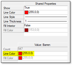
6

Click the small drop-down arrow and select a dark gray color. 2. 7

Click in the Fill Color field and select a medium gray color. 3. 8

Click Apply. The "Barren" class polygons change to gray. 4. 9

Change the Line Color and Fill Color properties for the remaining classes, using the screenshots below as a reference.

For the "Wetland" class colors, click the Custom tab in the color selection dialog and choose dark blue and cyan colors from the chart.

10

Click Apply. The class colors update in the Image window.

11

Click the Symbologydrop-down list and select Save/Update Symbology File. ENVI creates a Sentinel2_Montana_Classes.evs file in the same directory as the shapefile. As long as this .evs file stays in the same directory, ENVI will use it to display the appropriate colors when you open the classification shapefile in the future. 2. 12

This concludes the exercise.

In summary, supervised classifiers rely on training data to provide known examples of class data. The classifiers attempt to classify each pixel based on a similarity measure with the training class means. Depending on the classifier, the similarity measure can be Euclidean distance, standard deviation, probability, or spectral angle. In this quick guide, you visually compared the results of four different classifiers and created a Minimum Distance classification image.

For a more quantitative and scientific way to determine class accuracy, you can evaluate confusion matrices. See the Evaluate Class Statistics and Confusion Matrices quick guide for details.

Finally, you can use the Edit Classification Image tool to fix misclassified pixels when you are certain of their actual classes. See the Edit Classification Images quick guide for details.

Additional Resources

•

Collect Classification Training Data from Image Spectra quick guide * •

Edit Class Names and Colors quick guide * •

Edit Classification Images quick guide * •

ENVI Machine Learning Tutorial: Supervised Classification(opens in a new tab) (PDF) * •

Evaluate Class Statistics and Confusion Matrices quick guide * •

Perform an Unsupervised Classification quick guide

Your input is important to us, please take a few moments to fill out ourQuick Guide Feedback(opens in a new tab)form.