Evaluate Class Statistics and Confusion Matrices
Lesson content
Lesson 1 of 1
Evaluate Class Statistics and Confusion Matrices
In this quick guide, you will:
- •
Open and display a National Agriculture Imagery Program (NAIP) aerial orthophoto, a Region of Interest (ROI) with image-derived training data, and a classification image created from the orthophoto. * •
View basic and advanced class statistics: These include minimum/maximum/mean/standard deviation pixel values, covariance, correlation, pixel count, percentage per class, histograms, eigenvectors, and eigenvalues. * •
Create and view a confusion matrix and accuracy metrics.
Sample Data
Download sample data below. Then extract the contents of the .zip file to a local directory.
[NAIP_Classification.zip
2.3 MB
DownloadArrow down with horizontal line beneath it](assets/NAIP_Classification.zip)
Open and Display NAIP Images
- 1
Select File > Open from the Menu bar. An Open dialog appears. 2. 2
Go to the directory where you saved the sample data, and select all of the files. 3. 3
Click Open. The Select Base ROI Visualization Layer dialog appears. 4. 4
Select NAIP_Subset_SanAntonio.dat and click OK. The images are added to the Layer Manager and displayed in the Image window. First is a NAIP true-color image with 60 cm resolution. Overlaying the image are Regions of Interest (ROIs) with training data for five classes: Unclassified (mostly shadows), Water, Developed, Trees, and Ground Cover.

- 5
Uncheck the NAIP image in the Layer Manager to view a classification image of the same area. An Extra Trees machine-learning classifier created this image. The Classification Aggregation and Classification Smoothing tools were used to clean up the image.

For future reference, machine-learning classification tools are available after installation of the ENVI Deep Learning module. They are located in the Machine Learning folder of the Toolbox. You do not need ENVI Deep Learning or the machine-learning tools for this exercise.

View Class Statistics
- 1
In the search window of the Toolbox, enter statistics. 2. 2
Double-click the Class Statistics tool that appears in the search results. The Classification Input File dialog appears. 3. 3
Select NAIP_Classification_Residential.dat and click OK. The Statistics Input File dialog appears. 4. 4
Select NAIP_Subset_SanAntonio.dat and click OK. The Class Selection dialog appears. 5. 5
Use the Ctrl key to multi-select Water, Developed, Trees, and Ground Cover. For this exercise, we will ignore the Unclassified class.

- 6
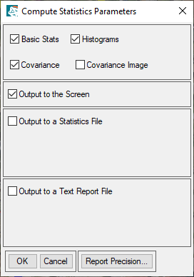
Click OK. The Compute Statistics Parameters dialog appears. 2. 7
Enable the Histograms and Covariance options. The Basic Stats and Output to the Screen options are enabled by default.
- 8
Click OK. The Classification Statistics View dialog appears.

View Basic Statistics
The Class Summary table shows the pixel count and percentage for each class, across all bands of the NAIP image (Red, Green, Blue, NIR).
The Class Means plot shows the mean brightness values of each class across all bands of the NAIP image. The mean values are also reported in tables for each class. For example, the Water table shows that the mean brightness value for the "Water" class is 149.22 in the Red band. Other basic statistics are also computed for each class such as minimum and maximum brightness values, and standard deviation.

View Class Histograms
- 1
Click the Select Plot drop-down list and select All Histograms Red. Histograms are plotted for each class, showing brightness values ("Data Value") and numbers of pixels ("Count") in the Red band of the NAIP image.

View Advanced Statistics
Each class has a series of tables for Covariance, Correlation, Eigenvectors, and Eigenvalues.
- 1
Scroll past the Basic Stats table for the "Water" class, and review the information in each table.

These statistics describe class variability with respect to NAIP image bands. A more common approach is to evaluate inter-class variability and accuracy using a confusion matrix. You will compute confusion matrices and accuracy metrics next.
- 2
Close the Classification Statistics View dialog.
Evaluate Class Accuracy Metrics
- 1
In the search window of the Toolbox, enter matrix. 2. 2
Double-click the Confusion Matrix Using Ground Truth ROIs tool that appears in the search results. The Classification Input File dialog appears. 3. 3
Select NAIP_Classification_Residential.dat and click OK. The Match Classes Parameters dialog appears.
The Matched Classes section shows the names of ground truth (training) ROIs, while the right side shows the class names. The ROI and class names are already paired, so you do not need to do anything further.
However, the Background ROI needs to be paired with an output class. ENVI automatically determines that "Unclassified" is the target class. 4. 4
Click Background. The "Background" ROI is added to the Ground Truth ROI field. 5. 5
Click Unclassified. The "Unclassified" class is added to the Classification Class field.

- 6
Click the Add Combination button. The Background <-> Unclassified pair is added to the Matched Classes list. 2. 7
Click OK. The Confusion Matrix Parameters dialog appears. 3. 8
Uncheck the Pixels option. You will evaluate percentages only. 4. 9
Keep the default selection of Yes for Report Accuracy Assessment.

- 10
Click OK. The Class Confusion Matrix dialog appears. The report consists of a confusion matrix and accuracy metrics.
Confusion Matrix
A confusion matrix compares the true classes in an image (based on the training data you provide) with the predicted classes. The confusion matrix presented here is wrapped across multiple lines, which makes it difficult to interpret. The "Unclassified" row is also duplicated.

Here is a different view that is easier to interpret:

The values along the diagonal (highlighted in yellow, for illustration) are the numbers of pixels where the ground truth and image classification agreed. In this example, 11,600 pixels were correctly classified as Trees.
A confusion matrix also provides more specific details on how well a classifier performed. Let’s look at some of these metrics.
Kappa Coefficient and Overall Accuracy

The Kappa coefficient is a measure of how well the classifier performed with respect to random data. It is an outdated metric that has little bearing on classification accuracy. The global, or overall, accuracy is of more interest. Overall accuracy is calculated by summing the number of correctly classified pixels and dividing by the total number of ground truth pixels in the image.
Overall accuracy only provides an initial, general estimate of how well a classifier performed. An accuracy of 97.6% seems great; however, keep in mind that this assessment doesn’t account for subtle differences between classes. Information located throughout the rest of a confusion matrix can provide more details on the relationships between classes. We will look at some of these metrics next.
Errors of Commission
These represent the fraction of values that were predicted to be in a class but do not belong to that class. They provide a measure of false positives. Errors of commission are shown in the rows of the confusion matrix, excluding the values along the diagonal. They are also reported in a separate table in the Class Confusion Matrix dialog, both as percentages and as numbers of pixels.

Errors of Omission
These represent the fraction of values that belong to a class but were predicted to be in a different class. They are a measure of false negatives. Errors of omission are shown in the columns of the confusion matrix, excluding the values along the main diagonal.

Producer Accuracy
This is the probability that a value in a given class was classified correctly.

User Accuracy
This is the probability that a value predicted to be in a certain class really is that class. The probability is based on the fraction of correctly predicted values to the total number of values predicted to be in a class.

For more information on interpreting these metrics, refer to the Calculate Confusion Matrics(opens in a new tab) topic in ENVI Help.
This concludes the exercise.
Additional Resources
- •
ENVI Machine Learning Tutorial: Supervised Classification(opens in a new tab) (PDF) * •
Perform a Supervised Classification quick guide
Your input is important to us, please take a few moments to fill out ourQuick Guide Feedback(opens in a new tab)form.
© 2024 NV5 Geospatial Solutions, Inc. This information is not subject to the controls of the International Traffic in Arms Regulations (ITAR) or the Export Administration Regulations (EAR).