Iterators and Aggregator Nodes
Lesson content
Lesson 1 of 1
ENVI Modeler - Iterators and Aggregators
This quick guide provides a more advanced overview of the ENVI Modeler. You will learn how to use Iterator nodes and Aggregator nodes to perform batch analyses that loop over multiple input datasets or multiple processing parameters. You will use these models to test different filter parameters, apply filters to several rasters, and create raster series and layer stacks of the filtered products.
You can find introductory concepts and examples in the Introduction to ENVI Modeler, Creating a Simple ENVI Model, andExporting ENVI Modelsquick guides. It is recommended that you complete those quick guides before starting this one.
This quick guide walks through three example use cases:
- Iterating a single process with different parameters.
- Iterating a single process for multiple files.
- Iterating a process for multiple files and aggregating the results.
Background
The following sections describe the purpose and uses of Iterator and Aggregator nodes in ENVI Modeler.
Iterator Nodes
Iterator nodes can be used to batch-process multiple datasets or loop through groups of elements, similar to using a FOR statement in IDL programming.
Example applications include:
- Applying the same operation on multiple rasters.
- Applying the same operation using a series of different parameters.
- Batch processing data on different ENVI Servers(opens in a new tab).
Note: nested iterations (loops) are not supported. To perform this kind of operation, you must close the first loop with an Aggregator node and pass the output to another Iterator node for the second loop.
Filter Iterator Nodes
Filter Iterator nodes can be used to apply conditional statements, similar to using IF...THEN statements in IDL. The nodes will iterate through the data while applying the specified condition.
You can add two Filter Iterator nodes in order to execute an IF...ELSE...THEN condition.
Note: use the Band Math task node to apply conditional operators to raster data values(opens in a new tab).
Aggregator Nodes
Aggregator nodes can be used to:
- Collect separate items into a single array that can be passed to a subsequent operation.
- Close a loop defined by an Iterator node.
Aggregator nodes are typically used in models containing iterator nodes. Additionally, Aggregator nodes are needed before task nodes that require an array of input rasters, like the Build Time Series task.
Aggregator nodes can take many inputs, but they must be of the same data type, for instance, raster or vector. However, Aggregator nodes will not accept other inputs when they are used to close iterator loops. To combine the outputs from several loops, you can link multiple Aggregator nodes.
Sample Data
You will explore and run models using four pre-processed Synthetic Aperture Radar (SAR) intensity images from the European Space Agency's Sentinel-1 satellite, covering a flood event in Cairns, Australia, in December 2023. SAR image preprocessing was carried out using ENVI SARscape and involved:
- Multi-looking: resampling to reduce noise,
- Coregistration: resampling of all images to a reference image, in this case the first date,
- Filtering: to reduce noise further,
- Geocoding: transformation from SAR coordinates to geographic coordinates.
The ENVI SARscape outputs, which have units of decibels, were saved as ENVI-format rasters and can be visualized in ENVI without requiring additional module licenses.
The sample dataset will allow you to observe changes in backscatter due to variable soil moisture in areas with farmlands. Since standing water has low backscatter, you will also be able to identify flooded areas in the December 16, 2023 image based on the reduction in backscatter compared to the other dates without floods.
Sample Data Download
Download the ZIP file below, and extract the contents to a directory on your system.
[S1_Flood.zip
400.8 MB
DownloadArrow down with horizontal line beneath it](assets/S1_Flood.zip)
First, open the dataset in ENVI:
- 1
From the Menu bar, select File > Open. An Open dialog appears. 2. 2
Go to the directory where you saved the files for this tutorial. 3. 3
Click each .dat file while holding down the Ctrl key to highlight all five files. Then click Open. The Sentinel-1 rasters are displayed in the Image window.
Example 1 - Iterate a Single Process with Different Parameters
In this example, we will illustrate how to import a single raster, apply a filter using different window sizes, and save the outputs with the appended parameter value to compare the results.
You can download the ENVI Model for this example here:
[Model1_FilterTests.model
3.8 KB
DownloadArrow down with horizontal line beneath it](assets/Model1_FilterTests.model)
- 4
Download the model using the link above and save it to your local files. 2. 5
Drag and drop the model file into ENVI. This opens up the model in the ENVI Modeler window. Alternatively, open the Modeler window (Display > ENVI Modeler), then open the model from the window (File > Open).
The model looks as follows:

This model accepts an Input Raster using the pink Input Parameters node, which it feeds to the Enhanced Frost Adaptive Filter node. It also uses an Array of Valuesnode (cyan) that has been set to values of 3, 6, and 9. These will be the window sizes that we loop through for the Filter task. Using the Iterator node between the Array of Valuesand Enhanced Frost AdaptiveFiltertask node ensures that the task will be ran once using each of those values as the chosen window size. We have an additional task node, Generate Filename, which ensures that the output of each iteration has the window size value appended to the filename so we can keep track of which output is which.
This example uses anEnhanced Frost Adaptive Filter, which has four parameters that can be adjusted: Window Size, Damping Factor, Homogeneous Cutoff and Heterogeneous Cutoff. You can find more information about the different types of adaptive filters and their parameters in the ENVI Documentation Center(opens in a new tab).
The following video walks you through the parameters and connections in this model:


Video Player is loading.
Play Video
Play
Loaded: 0%
0:00
Remaining Time --:-
1x
Playback Rate 1x
- 2x
- 1.75x
- 1.5x
- 1.25x
- 1x, selected
- 0.75x
- 0.5x
- 0.25x
Captions
- captions off, selected
Picture-in-PictureFullscreen
Mute
This is a modal window.
The main items to note are:
- •
Each value for the Array of Valuesnode is provided on its own line and the Data Type is set to Integer * •
The connection between the Iterator node and the Filter task node uses the Output from theIterator and not the Iteration Index. This is because we want to use the provided integer values of 3, 6, and 9 as the window sizes, and not the value of iteration, which would instead be 0, 1, and 2. * •
Similarly, the connection between the Iterator node and the Generate Filename task node uses the Output from theIterator and not the Iteration Index. Again, we want the provided integer to be appended to the filename, and not the iteration number. * •
The Generate Filename task node has a preset Filename Prefix that you can modify, and optionally, change to be one of the inputs you provide through the Input Parameters node. The Append Random Number option is set to No, such that the appended number is the one provided by the iterator and not a random one.
Save, Validate, and Run the Model
The model is ready to run. It is always a good idea to save your model before running it, so you don't lose your progress if the program crashes.
- 1
Save the model using File > Save As. 2. 2
Validate the model using Code > Validate Model. 3. 3
Run the model using Code > Run Model.
Since this model has anInput Parameters node, you will see a dialog prompting you to select the Input Raster and set a Directory for the outputs. 4. 4
Click on the ellipsis next to Input Raster. This opens up the Data Selection dialog.
Since you previously opened up the 5 rasters earlier, you will see these show up in this dialog. 5. 5
Select the sentinel1_20231110_dB.dat file and click OK. 6. 6
Click the ellipsis next to Output and navigate to the directory where you want to save the outputs from this model. 7. 7
Click OK to run the model.
When you run a model, the cells turn grey, then yellow as they are in progress, and green once completed. The Iterator task remains yellow as all three iterations are happening, and the Filter task flashes yellow then green multiple times as the processing is completed for each parameter that is iterated through.
After the model runs, three output files are added to the Layer Manager and displayed in the Image window, above the 5 original rasters.

You can zoom in to different parts of the image and check and uncheck the three layers to compare the effect of increasing the Enhanced Frost Filter window size. Comparing the outputs in an area with clear edges—like the coastline or around water bodies—shows that the larger the window size, the less detail is preserved.
This concludes the first example. The second example will show you how to apply this filter in bulk to all input rasters.
Example 2 - Iterate a Single Process for Multiple Files
In this example, we will illustrate how to import all five Sentinel-1 rasters and apply the Enhanced Frost Filter, making use of an Iterator node. The procedure is similar to that for the previous model, but this time you do not need an Array of Values node.
You can download the ENVI Model for this example here:
[Model2_FilterSAR.model
3 KB
DownloadArrow down with horizontal line beneath it](assets/Model2_FilterSAR.model)
- 1
Download the model using the link above and save it to your local files. 2. 2
Drag and drop the model file into ENVI. This opens up the model in the ENVI Modeler window. Alternatively, open the Modeler window (Display > ENVI Modeler), then open the model from the window (File > Open).
The model looks as follows:

- 3
Click on the bottom right icon on the blue Rasters node. This brings up the Data Selection dialog, showing the 5 opened rasters. 2. 4
Click Select All, to highlight all 5 files.

- 5
Click OK to dismiss the dialog. The cyan node will be renamed5Rasters.
The main items to note are:
- •
The Input Rasters are connected directly to the Iterator node in this example. This is because we are performing a single operation, filtering, on each of the input files, one by one. * •
There is an additional node, Extract Properties and Metadata, before the Generate Filenames node.
This task allows you to extract metadata from a file to be used as an input to another node. In our case, we want to extract the acquisition time for each of the images to be used as the prefix for the output files, such that we can keep track of which filtered output corresponds to which date.
As shown below, the acquisition time from the Extract Properties and Metadata node is therefore set as the Filename Prefix for the Generate Filename node.

- •
The Filter task has the Iterator output as the Input Raster, all other parameters as default, and the Generate Filename output as the Output Raster.

Save, Validate, and Run the Model
- 1
Save the model: File > Save As. 2. 2
Validate the model: Code > Validate Model. 3. 3
Run the model: Code > Run Model or select the Run icon on the toolbar.
Tip: If you select Code > Run Model in Debug Mode, you can see the timing of different process nodes.
The cells initially turn grey, then yellow as they are in progress, and green once completed. The Iterator task remains yellow as all three iterations are happening, and the Enhanced Frost Adaptive Filter task flashes yellow then green multiple times as the processing is completed for each parameter that is iterated through.
The files are added to the Layer Manager and displayed in the Image window.
This concludes the second example. The third example extends this model to create a raster series with the outputs.
Example 3 - Iterate a Process and Aggregate the Results
In this example, we will illustrate how to aggregate the results from an iteration to create a raster series and layer stack that you can save to a file and visualize in ENVI. The layer stack will allow you to visualize changes in SAR intensity for selected pixels over time.
You can download the ENVI Model for this example here:
[Model3_SARseries.model
7 KB
DownloadArrow down with horizontal line beneath it](assets/Model3_SARseries.model)
- 1
Download the model using the link above and save it to your local files. 2. 2
Drag and drop the model file into ENVI. This opens up the model in the ENVI Modeler window. Alternatively, open the Modeler window (Display > ENVI Modeler), then open the model from the window (File > Open).
The model looks as follows:
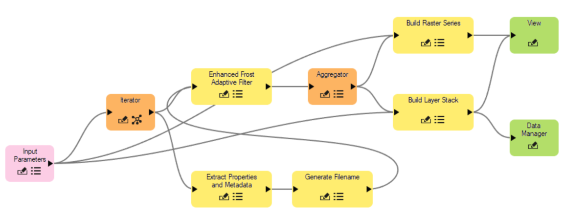
The main items to note are:
- •
The Input Parameters node is set to take the Input Rasters, the output directory for the Raster Series output (Output Raster Series URI), and the output directory for the Layer Stack (Output Raster URI). * •
Since the input to the Iterator node is a not yet defined raster provided by the Input Parameters node, the Extract Properties and Metadata node does not have a populated Known Properties list, and you must therefore include the name of the field to extract under Other Properties:

- •
The Aggregator node is placed after the tasks that the iterative operation is carried out on. In this case there is a single Filter task. If there was an additional task to carry out on each individual filtered image, this task would be placed before the Aggregator node, as the Aggregator node sets the end of the loop. * •
The Layer Stack will be shown in the ENVI view but also loaded to the Data Manager.
Save, Validate, and Run the Model
The model is ready to run:
- 1
Save the model: File > Save As. 2. 2
Validate the model: Code > Validate Model. 3. 3
Run the model: Code > Run Model or select the Run icon on the Toolbar.
Since the model has an Input Parameters node, a dialog appears, prompting you to enter theInput Rasters, Output Raster Series, and Output Raster:
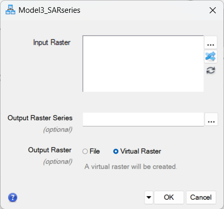
- 4
Click the ellipsis next to Input Raster to select the inputs. A Data Selection dialog appears. 2. 5
Since your five Sentinel-1 rasters are already open in ENVI, they will show up under Select Input Data. You can click the Select All button to select all. If your files are not already loaded into ENVI, you can click the Open File icon to navigate to the directory where you saved the data and open the files from there.

- 6
Click OK to dismiss the dialog. 2. 7
Click on the Sort icon (blue arrows) next toInput Raster to sort the inputs by date.
Note: the Layer Stack task will stack the layers in the order they are provided to the task. In order to produce a usable time-series, you will need to sort the layers by date. 3. 8
Click the ellipsis next to Output Raster Series to select a directory and file name, for instance S1_Flood.series, for the output series. The appropriate extension for a series file is .series. 4. 9
Select the File option next to Output Rasterand click the three dots to select a directory and file name, for instance S1_Flood_stack.dat, for the output layer stack.

- 10
Click OK to dismiss the dialog.
Once you set the Input Parameters and click OK, the model runs as shown in the video clip below:


Video Player is loading.
Play Video
Play
Loaded: 0%
0:00
Remaining Time --:-
1x
Playback Rate 1x
- 2x
- 1.75x
- 1.5x
- 1.25x
- 1x, selected
- 0.75x
- 0.5x
- 0.25x
Captions
- captions off, selected
Picture-in-PictureFullscreen
Mute
This is a modal window.
Visualize the Model Outputs
The ENVI Layer Manager and Image window show the time-series and layer-stack output.
As noted in the Sample Data section above, this dataset showcases more subtle changes in SAR backscatter due to variable soil moisture in farmlands as well as a stronger change due to flooding.
You can use the Series output to visually inspect these changes over the five dates. Notice the appearance of dark (low backscatter) pixels around the rivers on the December 16, 2023 image, due to the floods.
- 1
Display the Series Manager by selecting Display > Series/Animation Manager from the Menu bar. 2. 2
Click the blue forward arrow to play through the images, one by one. You can adjust the display time from the 0.1 sec default to 0.5 or 1 sec.
The video clip below shows the Series Manager output. Notice the change in intensity for the individual land patches in the lattice of farmland parallel to the shore. Also notice how the area around the river in the bottom-right part of the image turns black on the 16 December 2023 image - this is the location of the standing flood water.


Video Player is loading.
Play Video
Play
Loaded: 0%
0:00
Remaining Time --:-
1x
Playback Rate 1x
- 2x
- 1.75x
- 1.5x
- 1.25x
- 1x, selected
- 0.75x
- 0.5x
- 0.25x
Captions
- captions off, selected
Picture-in-PictureFullscreen
Mute
This is a modal window.
- 3
Close the Series Manager. 2. 4
Uncheck the Series file in the Layer Manager to view the Layer Stack.
The layer-stack raster is displayed as a Red-Green-Blue (RGB) composite using the first three dates for each color channel. Notice how the farmlands appear in shades of blues, reds, yellows, greens and purples. This is because of the changing intensity from variable soil moisture in the first three dates.
You can open the Data Manager to load individual images as Grayscale images, or to select a different group of images to visualize as an RGB composite. You will do this next.
- 5
Select File > Data Manager from the Menu bar. 2. 6
Under the layer-stack file in the Data Manager, click the 20231110 image, then the 20231216 image, then the 20231228 image, then click Load Data.
This brings up a new image where the red channel shows the pre-flood date intensity, the green channel shows the flood date intensity and the blue channel shows the post-flood date intensity.
Since flooded areas have low SAR intensity, flooded areas show up in purple tones (high intensity in the red and blue channels, low in the green).
You can use the Spectral Profile tool, marked with the red box in the image below, to view a profile of the SAR amplitude for single pixels in the image over the five stacked dates:

You can click around the image to see how the intensity changes over time for different locations in your image.
If you click on a pixel in the flooded area, you will see that Index 4, corresponding to the flood date of December 16, 2023 has the lowest Intensity (around -15 to -20 dB), as shown in the image below:

This concludes this quick guide.
Your input is important to us, please take a few moments to fill out ourQuick Guide Feedback(opens in a new tab)form.
© 2024 NV5 Geospatial Solutions, Inc. This information is not subject to the controls of the International Traffic in Arms Regulations (ITAR) or the Export Administration Regulations (EAR).